In a previous post we considered using R to fit one-way ANOVA models to data. In this post we consider a few additional ways that we can look at the analysis.
Fast Tube by Casper
Fast Tube by Casper
In the analysis we made use of the linear model function lm and the analysis could be conducted using the aov function. The code used to fit the model is very similar:
> plant.mod2 = aov(weight ~ group, data = plant.df) > summary(plant.mod2) Df Sum Sq Mean Sq F value Pr(>F) group 2 3.7663 1.8832 4.8461 0.01591 * Residuals 27 10.4921 0.3886 --- Signif. codes: 0 ‘***’ 0.001 ‘**’ 0.01 ‘*’ 0.05 ‘.’ 0.1 ‘ ’ 1 |
The output from using the summary function of the fitted model object shows the analysis of variance table with the p-value showing evidence of differences between the three groups. In R we can investigated the particular groups where there are differences using Tukey’s multiple comparisons:
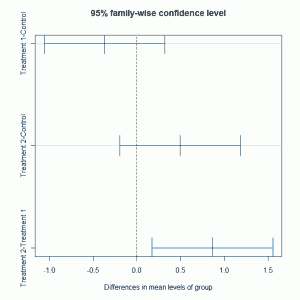
> TukeyHSD(plant.mod2) Tukey multiple comparisons of means 95% family-wise confidence level Fit: aov(formula = weight ~ group, data = plant.df) $group diff lwr upr p adj Treatment 1-Control -0.371 -1.0622161 0.3202161 0.3908711 Treatment 2-Control 0.494 -0.1972161 1.1852161 0.1979960 Treatment 2-Treatment 1 0.865 0.1737839 1.5562161 0.0120064 |
The multiple comparison tests highlight that the difference is due to comparing treatments 1 and 2. These 95% confidence intervals for the differences shown above can be plotted:
plot(TukeyHSD(plant.mod2)) |
which gives
The post-hoc adjustments are recommended as we are testing after looking at the data rather than undertaking a pre-planned analysis.


How interesting. Intuitively I would say control2 and treatment don’t look all that different.