A 3d wireframe plot is a type of graph that is used to display a surface – geographic data is an example of where this type of graph would be used or it could be used to display a fitted model with more than one explanatory variable. These plots are related to contour plots which are the two dimensional equivalent.
To illustrate this type of graph we will consider some surface elevation data that is available in the geoR package and was used in the blog post on level plots. The data set in this package is called elevation and stores the elevation height in feet (as multiples of ten feet) for a grid region of x and y coordinates (recorded as multiples of 50 feet). This post has details of the various operations that are undertaken to prepare the data for graphing.
Base Graphics
Fast Tube by Casper
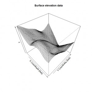
The function persp is the base graphics function for creating wireframe surface plots. The persp function requires a list of x and y values covering the grid of vertical values which is specified as the z variable. The heights for the display are specified as a table of values which we saved previously as the object z during the calculations when the local trend surface model was fitted to the data. The text on the axis labels are specified by the xlab and ylab function arguments and the main argument determines the overall title for the graph.
persp(seq(10, 300, 5), seq(10, 300, 5), z, phi = 45, theta = 45, xlab = "X Coordinate (feet)", ylab = "Y Coordinate (feet)", main = "Surface elevation data" ) |
The function arguments phi and theta are used to rotate the viewing angle of the surface. Trial and error is probably the way to go when setting these as good choices depend entirely on the shape of the surface being displayed.
The surface is clear and easy to determine the shape and variation in height across the x and y grid coordinates.
Lattice Graphics
Fast Tube by Casper
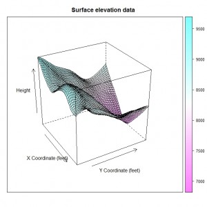
The lattice graphics package has a function wireframe and we use the data in the object elevation.fit to create the graph. We use the formula interface to specify first the z axis data (the heights) followed by the two variables specifying the x and y axis coordinates for the data.
wireframe(Height ~ x*y, data = elevation.fit, xlab = "X Coordinate (feet)", ylab = "Y Coordinate (feet)", main = "Surface elevation data", drape = TRUE, colorkey = TRUE, screen = list(z = -60, x = -60) ) |
The axes labels and title are specified in the same way as the base graphics with the xlab, ylab and main function arguments. A colour key is added using the colorkey function argument and setting it to TRUE.
The surface produced by the wireframe function is similar to the persp function with the main difference between the colours used on the surface.
This blog post is summarised in a pdf leaflet on the Supplementary Material page.


“display a fitted model with more than one explanatory variable”
I am very curious to see how such graphs could be used to interpret a fitted model. Do you think you could come up with an example? Thank you
Getting this error
“Error in persp.default(seq(10, 300, 5), seq(10, 300, 5), z, phi = 45, :
invalid ‘z’ argument”
The object z needs to be created first to be used for the perspective plot. The details of preparing the data for this type of graph are in the blog post on level plots linked at the start of this one. Take a look at the steps I followed there are see if that can solve your problem.
When the last graphic appears, it’s all black wothout colors just black. What happen?
Can you make a for loop with the wireframe function, creating a rotating plot, like you can do with the cloud function?
You might be able to although it would appear that the rgl package is probably more to your requirements?
An alternative would be to create a series of statistic images and then wrap them together into an animated graphics file.
Hope that helps.
Hi,
I am getting:
Error in persp.default(seq(10, 300, 5), seq(10, 300, 5), z, phi = 45, :
invalid ‘z’ argument
I prepared the data as described here:http://www.wekaleamstudios.co.uk/posts/displaying-data-using-level-plots/
The level plot is working out fine.
Apprecitae the help and thanks
P
Hi,
I getting the same message like Rae:
Error in persp.default(seq(10, 300, 5), seq(10, 300, 5), z, phi = 45, :
invalid ‘z’ argument
…although I prepared the data accordingly.
Also, like Sacramento says, in the last graph the surface appears all black without colours.
Help would me much appreciated.
Hi Rae and Noralf,
I think that I have identified the problem. The dimensions of z are different to the range of values created for x & y using seq(10, 300, 5) so that is why persp is not working correctly.
Try running:
> dim(z)
x y
291 291
> length(seq(10, 300, 5))
[1] 59
and you will see what I mean.
One way that I found to fix it is to replace ‘5’ with ‘length.out=291’ in the two seq commands to get:
persp(seq(10, 300, length.out=291), seq(10, 300, length.out=291),
as.matrix(z), phi = 45, theta = 45,
xlab = “X Coordinate (feet)”, ylab = “Y Coordinate (feet)”,
main = “Surface elevation data”
)
Hope this helps,
Ralph
Hi Ralph,
Thank you! Works now. When I solved the “black surface” problem I’ll post it here.